Dynamic
variables and parameters
Bifurcation
diagrams
Time
scales and adiabatic systems
Bifurcations
and hysteresis
Scaling laws
Let us consider a dynamical system, described either by an ordinary differential equation, or by an iterated map. Such a system depends usually on two kinds of variables: dynamic variables and parameters. Dynamic variables evolve in time, specify the state of the system at each instant, and determine the future evolution. Parameters also influence the dynamics, but they remain fixed. Let us consider two examples:
Example 1: A thin layer of fluid is contained between two horizontal plates. The lower plate is kept at a higher temperature than the upper plate. This experiment is known as Rayleigh-Bénard convection. At least when the temperature difference is not too large, and there is no turbulence, the system can be described approximately by an ordinary differential equation. The dynamic variables are amplitudes of the dominant Fourier modes of the velocity and temperature fields, and the parameter is the temperature difference between the plates.
Example 2: In small ecosystems, the dynamics of competing populations can sometimes be described by an iterated map. The dynamic variables are the number of individuals of each competing species (e.g. predator and prey), while the meteorological or climatic conditions (averaged on a reproduction cycle) can be considered as parameters.
Dynamical systems are sometimes characterised by a bifurcation diagram. It represents the asymptotic state of the system as a function of the parameter. This diagram can be determined experimentally in the following way:
Consider for instance the convection experiment of Example 1. First, we have to fix the temperature difference. Then we have to wait for the system to reach an asymptotic state (this state is stationary for small temperature difference). After measuring the characteristics of this state, we should repeat the experiment for a different initial condition, i.e. by stirring the fluid a little bit. This whole procedure should then be repeated for another value of the temperature difference, and so on, until we have enough data to draw the characteristics of the asymptotic state (e.g. the rotation frequency of convection rolls) as a function of the parameter.
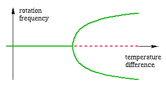
In Example 1, the following diagram is obtained: for small temperature difference, the asymptotic rotation frequency is zero, regardless of the initial condition, in other words, there are no convection rolls. For larger temperature difference, there are two possible asymptotic states, with positive or negative rotation frequency. The choice of the asymptotic state depends on the initial condition. The transition between both regimes is called a pitchfork bifurcation (Fig.1).

Figure 1: A pitchfork bifurcation, as it is observed, for instance, in Rayleigh-Bénard convection. When the temperature difference is small, the asymptotic rotation frequency is zero, there is no convection (green line). For a larger temperature difference, this state becomes unstable (red dotted line), and two new stable equilibria appear, which describe convection rolls with positive and negative rotation frequency.
Similar phenomena can be observed in Example 2: for instance, by changing the reproduction rate of the prey, one can pass from a stationary asymptotic state to a state of period two, in which the number of individuals oscillates between two values from one cycle to the next (period doubling bifurcation).
The procedure for determining the bifurcation diagram can take a long time, since we have to wait for the system to reach equilibrium for each value of the parameter, and reset the initial condition. One could be tempted to modify the parameter slowly during the experiment, in the hope that this will not affect the bifurcation diagram. But first of all, what do we mean by slowly?
A dynamical system can be characterised by different time scales. They are determined, for instance, by the period of a typical periodic orbit, or the rate of exponential relaxation to equilibrium. In Example 1, we could take the period of revolution of a convection roll as time unit (a few seconds). In Example 2, a possible time unit is the duration of one reproduction cycle of the predator (depending on the species, this can represent a few days or a year).
We call adiabatic system the system obtained by varying the parameter, say, periodically, with a period equal to ε - 1 times a typical time scale of the system with frozen parameter, where ε is a small number called the adiabatic parameter. This parameter will be treated as a small quantity in the perturbative analysis. Mathematically speaking, this is a singular perturbation problem, which has to be handled with some care. One can, however, obtain precise result, assuming that ε is sufficiently small.
Thus, in Example 1, we are in the adiabatic regime if the temperature difference between the plates oscillates with a period of several minutes. In Example 2, if the predators reproduce every year, a climatic change extending over several generations can be considered as adiabatic.
If the family of static dynamical systems admits a stable equilibrium, depending smoothly on the parameter, solutions of the adiabatic system will follow this equilibrium at a small distance (of order ε). Such a behaviour is also called quasistatic in thermodynamics. Thus, varying the parameter back and forth will only cause the system to oscillate close to this equilibrium, and there are no memory effects.
The situation changes drastically in presence of bifurcations. At a bifurcation point, several equilibrium branches may meet, causing the system to choose between several directions. Consider for instance the pitchfork bifurcation of Example 1: when the parameter crosses its critical value, the system has to choose between its current, unstable position, and the two new stable equilibria. The actual behaviour of the system is quite surprising: it remains for some time close to the unstable origin, before jumping on one of the branches. This phenomenon of bifurcation delay can be considered as a kind of metastability.
When the parameter is varied back and forth, the system does not always follow the same equilibrium branch for a given value of the parameter, in other words it displays hysteresis. In the language of the convection experiment, convection rolls appear suddenly, with a positive rotation frequency, at a higher temperature difference than the critical value. They disappear smoothly, after a slow deceleration, when the critical temperature difference is reached again (Fig. 2).
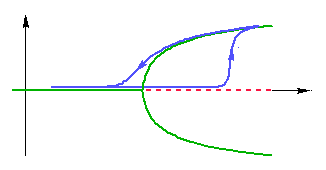
Figure 2: When the parameter of the example in Fig. 1 is varied periodically, the system displays hysteresis. This is due to the fact that when the parameter is increased, the asymptotic orbit stays for some time close to the unstable origin, before jumping on the stable branch, which it follows when the parameter is decreased again.
This motion is qualitatively equivalent to the overdamped dynamics of a particle in a potential of Ginzburg-Landau type, which varies between a single and a double well (Fig. 3). When the parameter is increased, the particle remains for some time in unstable equilibrium close to the maximum at the origin, before rolling into one of the wells. When the system is not overdamped, but includes inertia, the sequence of chosen wells may even be chaotic, a phenomenon that we called chaotic hysteresis.
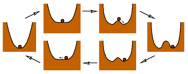
Figure 3: The bifurcation diagram of Fig. 1 and 2 also described the overdamped motion of a particle in a potential which oscillates between a single and a double well. For a given shape of the well, the asymptotic position of the particle is not always the same.
A more familiar example of hysteresis is the motion of a particle in a double-well potential with an external field. For intermediate values of the field, the position of the particle depends on the last attained threshold of the field, which forces the particle into one of the potential wells (Fig. 4).
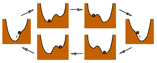
Figure 4: When an oscillating linear potential is added to the double well, the system displays another type of hysteresis. It is related to the fact that for sufficiently strong field, one of the wells disappears, and the particle rolls into the other one. It has to remain in this well until the field has attained another threshold value, which makes the well disappear.
One of the important properties of hysteresis cycles is the way there properties scale with the adiabatic parameter. It has been discovered that the area enclosed by the cycle follows a particular scaling law, with an exponent depending only on certain qualitative features of the bifurcations. For instance, with the example in Fig. 4 is associated the scaling law
A(ε) ~ A(0) + ε2/3.
The hysteresis cycle of Fig. 3 obeys another scaling law
A(ε) ~ A(0) + ε3/4.
Other exponent describe, for instance, the distance between the hysteresis cycle and its adiabatic limit. We showed that these exponents can be deduced in a simple way from the Taylor series of the vector field around bifurcation points.